SLV up 51% in 17 trading days. BOIL up 100+% in 5 trading days.
A stark reminder that often what we think is impossible in the market does end up happening. In a vacuum, these numbers look like glitches in the matrix, market errors that shouldn't exist.
Before we dive into the math, take a guess: Which of these two moves was statistically more unlikely?
Was it the 51% grind higher in Silver over three weeks? Or was it the sudden 100% explosion in Natural Gas in just one week?
If you ask a room of traders, most will pick SLV, as a confirmation of the recency biais: everybody is still amazed by the recent developments in the precious metals sector while BOIL being a leveraged ETFs and with a reputation to be explosive, it is almost expected to see such strong reaction.
Yet, they would be wrong. To understand why, we have to stop looking at return and start looking at volatility.
I. The Recipe: Normalizing Risk
The villain in this story is "Absolute Return Bias." A 100% return sounds like a winning lottery ticket. But return is just the numerator; risk (volatility) is the denominator. You cannot judge the speed of a car without knowing the speed limit on the road: doing 200 miles an hour downtown is clearly an outlier (and wrong by the way) but doing this on an F1 circuit is mandatory. The same idea, you cannot judge a return without knowing the variance required to get there.
To assess how "impossible" these moves were, we must normalize them. Crucially, we do not use long-term historical averages (like a 200-day average). Volatility clusters. When price explodes, volatility explodes alongside it. To get the truth, we must use the Realized Volatility (RV) specifically observed during the move.
Let’s run the numbers.
Case A: SLV – The "Fake" Outlier
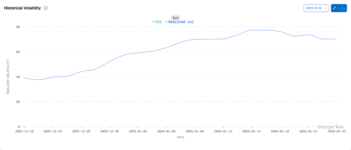
Silver has been on a tear, rallying 51% in 17 trading days.
- The Context: Over this specific 17-day period, SLV realized an annualized volatility of 70%.
- The Expectation: If we convert that 70% annual volatility down to a 17-day timeframe, the "standard" (1-sigma) expected move is roughly ±18.2%.
- The Verdict: Z-score: 51%/18.2% = 2.8 sigma
A 2.8-sigma event is rare, but it is not magic. Statistically, it happens roughly 0.5% of the time or once every year or two in volatile assets. The 51% return is impressive, but statistically, it was just a strong trend in a high-volatility environment. The high volatility explains the return almost perfectly.
Case B: BOIL – The True Outlier
Natural Gas went parabolic, rallying 100% in 5 trading days.
- The Context: Over this 5-day explosion, $BOIL realized a face-ripping 103% volatility.
- The Expectation: Converting 103% annual volatility to a 5-day timeframe gives us a standard expected move of ±14.5%.
- The Verdict: Z-score = 100%/14.5% = 6.9 sigma

This is where the math breaks. Even after adjusting for the massive 103% volatility, the price move still outpaced the risk model by a factor of seven.
In a normal Gaussian distribution, a 7-sigma event is statistically impossible (odds of 1 in billions). The fact that it happened is a stark reminder that financial markets have Fat Tails; extreme events happen far more often than models predict. But unlike Silver, this was a true statistical anomaly.
II. Visualizing the Extremes (Monte Carlo)
If the sigma math feels abstract, we can visualize it. We simulated 10,000 alternative realities using these specific volatility inputs (70% vs 103%) to see how often these moves actually happen in a random walk.
Visualization A: The Silver "Fan"
When we simulate Silver using 70% volatility, the "cone" of probability opens up wide.

Looking at the generated paths, you can clearly see a healthy cluster of orange lines (winning paths) crossing the +51% target line. The move looks aggressive, but it fits comfortably within the upper bound of the distribution. The simulation confirms the math: this was a "likely" outcome given the volatile environment.
Visualization B: The BOIL "Cloud"
The simulation for BOIL tells a violent story.

Even with the massive 103% volatility input, the grey cloud of 10,000 paths barely rises off the x-axis relative to the target. The +100% target line sits high above the density of the probability cloud. Likely zero or near-zero paths touch it. It effectively required a perfect storm to breach that level in just 5 steps.
The "Cataclysmic" Counterfactual
Why does normalization matter? Consider this:
If BOIL had displayed the volatility of a "boring" stock like Apple (~20%) instead of 103%, a 100% move in a week would be a 35-sigma event.
A 35-sigma event implies the market mechanics have ceased to function and you can throw every piece of modelization out of the window. A 7 sigma move starts calling the same question: many people will expect mean reversion or at least a non continuation of the moves. But until realized volatility drops, a lot of things are possible.
Finally, you haven’t seen a sudden margin increase from the different brokerages in BOIL: the reason is because the weekly volatility was already running at 101% before that week. High volatility was expected and acted as a shock absorber for the high return.
III. Did the Market See It Coming?
Retail traders are often shocked by these moves, but the options market is rarely caught completely off guard. We can check this by looking at Call Skew and Implied Volatility.

In commodities, "Positive Skew" means the market expects volatility to increase as price increases;in both cases, panic to the upside.
- In SLV: The 10-Delta Call IV was trading around 80%. This was actually remarkably accurate compared to the 70% realized volatility we observed. The market priced the risk well.
- In BOIL: The 10-Delta Call IV was screaming at 135%.
The market knew $BOIL was a powder keg. It was pricing in extreme variance.

However, this highlights a dangerous trap for option sellers. Even if you sold calls at 135% IV (expecting them to be overpriced), a 7-sigma move is functionally impossible to hedge perfectly. The velocity of the move (Gamma) would likely force a squeeze before you could adjust your delta hedges.
High Implied Volatility isn't "free money" for sellers; it is a neon sign reading "Danger Ahead."
Conclusion: The Relativity of Risk
So, which move was more surprising?
The answer is unequivocally BOIL.
- SLV 2.8 sigma: A "Fake" Outlier. The 51% return is impressive, but statistically, it was just a Tuesday in a 70% volatility regime.
- BOIL 7 sigma: A "Real" Outlier. A true fat-tail event where returns outran even the most extreme volatility expectations.
The next time you see a stock up 50% or 100%, resist the urge to judge it by the percentage alone. If you don't normalize by realized volatility, you aren't measuring performance—you are just measuring variance.
In the land of 100% volatility, a 100% return isn't a miracle. It’s just math. Adjust your expectations accordingly.