Why sell the call if its implied volatility looks cheap?

The put looks expensive. The call looks cheap. Sell both, and you seem to be giving back part of the advantage you found on the put.

That was the objection raised in our Discord recently. A member was comparing the implied volatility of each leg of a short strangle with a forecast of subsequent realised volatility. The put appeared to offer a premium. The call offered much less, perhaps none. Why include it?

As the discussion continued, the concern became more precise. Our assessment of volatility uses information from across the option chain. Our trade contains only two strikes. How much of the opportunity are we actually trading?

We include the call because it helps create the exposure we want: less bullish bias at entry, and sensitivity to volatility across a broader range of underlying prices. At Sharpe Two, where we trade these strangles without routine delta hedging, both contributions matter.

Different IVs, one underlying

An option's implied volatility is the volatility input that makes its pricing model reproduce its price. Different strikes can have different IVs for the same underlying and expiry. This is the volatility skew.

Consider these readings from Sharpe Two's modelled 30-day surfaces for 9 September 2026:

Underlying	20-delta put IV	ATM IV	20-delta call IV
SPY	16.91%	12.45%	10.25%
GLD	24.97%	25.12%	27.33%

Surface estimates for 15:50 New York time, retrieved on 10 September. These are reconstructed constant-tenor nodes, not executable quotes for particular contracts. Source: Sharpe Two analytics API.

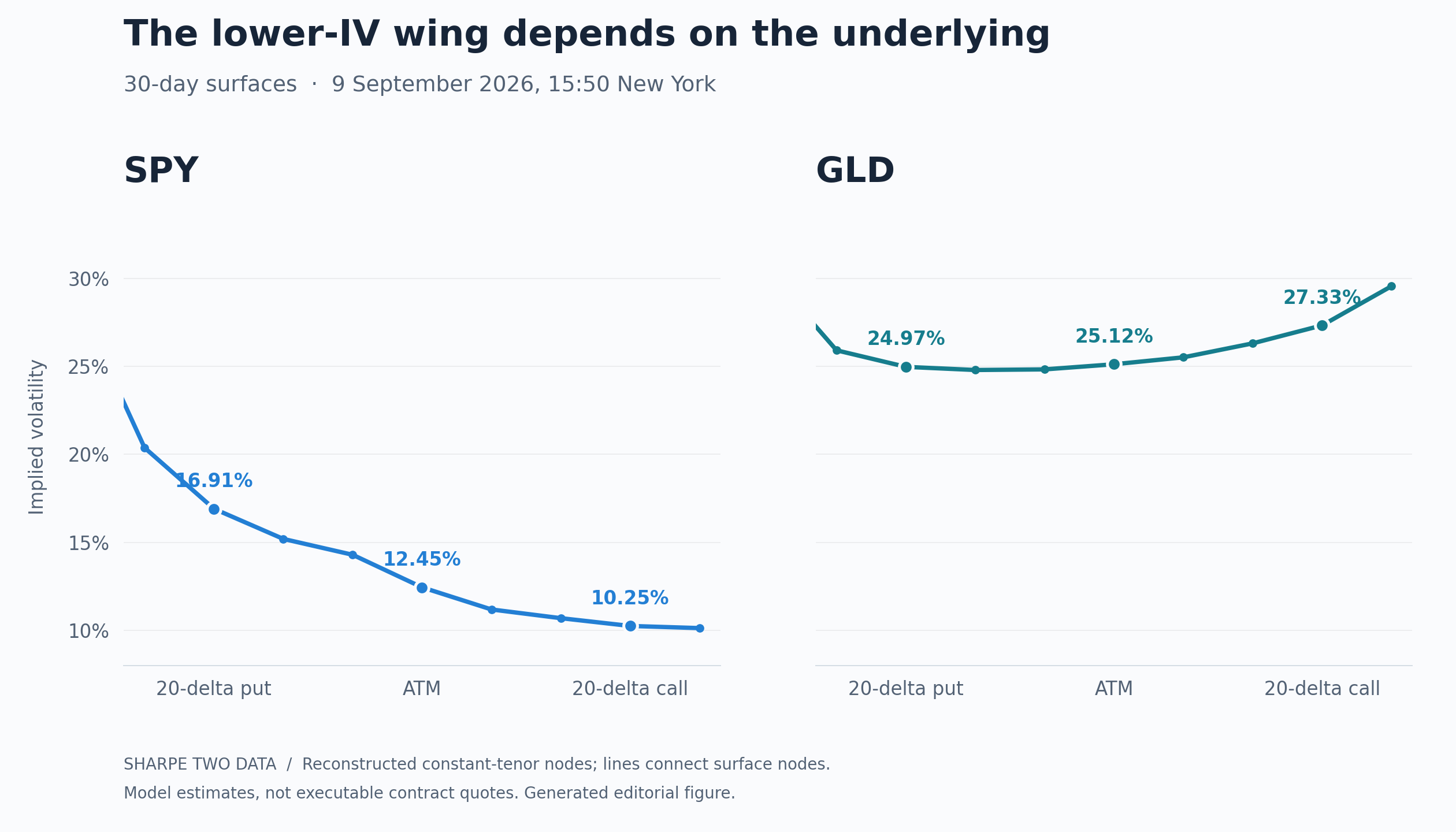
Sharpe Two’s reconstructed 30-day surfaces at 15:50 New York on 9 September 2026. SPY’s 20-delta put is at 16.91% IV and its call at 10.25%; GLD’s are 24.97% and 27.33%. Generated from the dated analytics API responses; lines connect modelled nodes, not executable quotes.

SPY shows the familiar equity pattern: the put has a substantially higher IV than the call. GLD's selected nodes show the reverse.

Both legs respond to the same underlying price process. The call does not experience a separate realised volatility because its quoted IV is lower. What differs is how each option responds to that process: its payoff, sensitivities and exposure to particular outcomes.

What can be misleading is the impression that each strike has its own separate realised-volatility outlook. Supply and demand for downside protection and upside exposure help shape option prices and their skew. IV translates those prices into a common volatility unit, making comparisons useful without creating a separate underlying price process for each leg. OIC explains how supply and demand contribute to volatility skew.

The IV quote remains meaningful: it expresses an option price in a common unit. Subtracting the same RV forecast from each leg's IV, however, does not give us two reliable estimates of expected profit. A forecast of overall movement does not specify the distribution of returns needed to value each payoff.

What the variance measure tells us

A variance swap settles against realised variance over a defined period. Its fair strike can be inferred, under standard replication assumptions, from a broad strip of option prices. In a discrete approximation, the option-price contributions have weights proportional to strike spacing divided by strike squared: ΔK/K².

This includes information from the wings that ATM IV leaves out. It also includes the market's compensation for bearing risk, so the resulting implied variance is not simply an unbiased forecast of what will happen. The replication and its limitations are developed by Demeterfi, Derman, Kamal and Zou.

In volatility units, the square root of that variance strike often sits above ATM IV on a skewed equity surface. That is not a defining inequality: in the ideal flat-volatility Black–Scholes case, the two coincide.

This broader measure helps us ask whether the market's pricing of future movement looks expensive against our forecast. It does not establish that every option in the chain is overpriced by the same amount.

Some premium may sit in far-out strikes that our strangle never sells. We cannot claim that premium merely because our signal includes it. Equally, averaging the put and call IVs does not recover the variance exposure of the combination. Even a single IV fitted to the combined premium would be a model-dependent price summary, not a forecast of the trade's return.

What the call changes

Suppose we sell one 20-delta put with a standard 100-share multiplier. Its initial delta is approximately +20 shares: a bullish position, whether or not we intended to express a directional view.

Selling a 20-delta call contributes approximately −20 shares of delta. The combination starts near zero. We collect another premium and add short gamma and short vega on the call side.

That balance changes. With other inputs fixed, a decline increases the short put's positive delta while reducing the call's negative delta. A rally does the reverse. The strangle develops exposure against a continuing move in either direction.

The call can contribute positively during a sell-off, although a rise in its IV can offset some of the benefit from falling spot. Its maximum profit is the premium received. Once it is effectively worthless, it provides little further offset to put losses. A sufficiently strong rally exposes us to unlimited losses on the call itself. OIC describes the short strangle's payoff and risks.

The alternative raised in the discussion was to sell the put and hedge its delta with the underlying. That offsets delta without adding the call's short gamma and vega. Maintaining the hedge as the put's delta changes requires further trading.

At Sharpe Two, we avoid routine delta hedging of these strangles. For the way we trade, repeated adjustments are too costly and too prone to execution errors. We accept the changing directional exposure and concentrate on finding sufficiently overpriced volatility.

The second strike matters after spot moves

Vega measures an option's sensitivity to implied volatility. It changes as the underlying moves.

An ATM straddle concentrates its exposure around one strike. A strangle distributes it across two. As spot approaches one strike and moves away from the other, their contributions change differently.

Take a simple European-option model: underlying price 100, flat 20% IV, 30 calendar days to expiry, zero rates and dividends. The 20-delta strangle's strikes are approximately 95.45 and 105.12. Compare its vega magnitude with an ATM straddle, setting each position's initial reading to 100%.

If spot falls to 96 with time and IV unchanged, the straddle retains about 76% of its original vega; the strangle retains about 88%. At spot 104, the figures are approximately 81% and 96%.

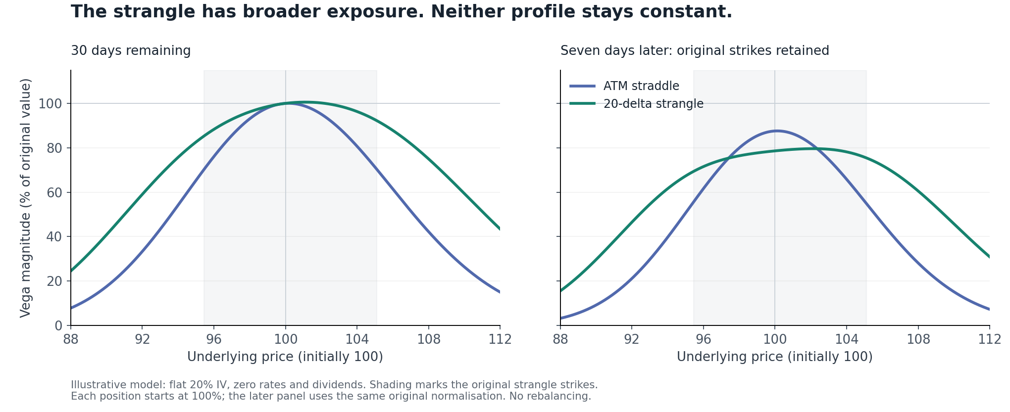
Illustrative Black–Scholes calculations. Each position is normalised to its own original vega magnitude. Strikes remain fixed; there is no rebalancing. These are sensitivity curves, not profit curves.

The strangle maintains a more even exposure across these spot levels. It still changes, including between the strikes. The second panel shows the effect of a week passing. An observed skew and changes in that skew add further differences.

The short straddle starts with more vega magnitude per pair in this model. It would gain more dollars from a small, immediate, parallel IV decline with spot unchanged. These are not comparisons at equal capital or risk. A flatter sensitivity curve alone cannot establish better returns or lower return variability.

The call gives us another strike around which to retain volatility sensitivity as spot moves. That is its contribution beyond the initial delta offset.

Turning the forecast into a trade

Our forecast asks whether current implied volatility is likely to exceed subsequent realised volatility over a corresponding horizon. That is the starting point for selection. The contracts, entry prices and risk we retain determine how we implement it.

One shorthand from the discussion needs care: P&L = (IV − RV) × vega. It is not an accounting identity for our unhedged strangle. Even in idealised delta-hedged option theory, the exposure to the implied-versus-realised variance difference is weighted by changing dollar gamma. Derman's volatility-trading notes show why the underlying's path matters.

For a European strangle held unchanged to expiry, the arithmetic is simpler. Before costs and financing, per unit of underlying:

P&L = total premium received − max(put strike − final spot, 0) − max(final spot − call strike, 0).

A choppy path that finishes between the strikes and a persistent move that finishes beyond one strike can produce very different results, even with similar measured RV. Before expiry, the path also affects valuation and margin. A correct volatility forecast can therefore accompany a losing trade.

Our unhedged strangle does not reproduce a variance swap's settlement. Ideal variance replication requires a broad option strip and dynamic trading in the underlying, under specific assumptions. Hobson and Klimmek explain the complications introduced by jumps and discrete monitoring.

A high variance signal warrants investigation; actual contract pricing can still make us pass. Establishing how reliably the signal translates into strangle returns requires results from that implementation, including costs.

We sell the call when its premium and contribution to the whole position justify the upside risk. Its IV can be lower than the put's and still meet that test.

In Sharpe Two, use the forecast and surface to identify the opportunity, then examine the contracts available to you: their combined premium, exposure as spot moves, and losses you would need to withstand. That is how we decide whether the call belongs in the trade.