SPY’s quiet rally: what happens after a big move with little volatility?

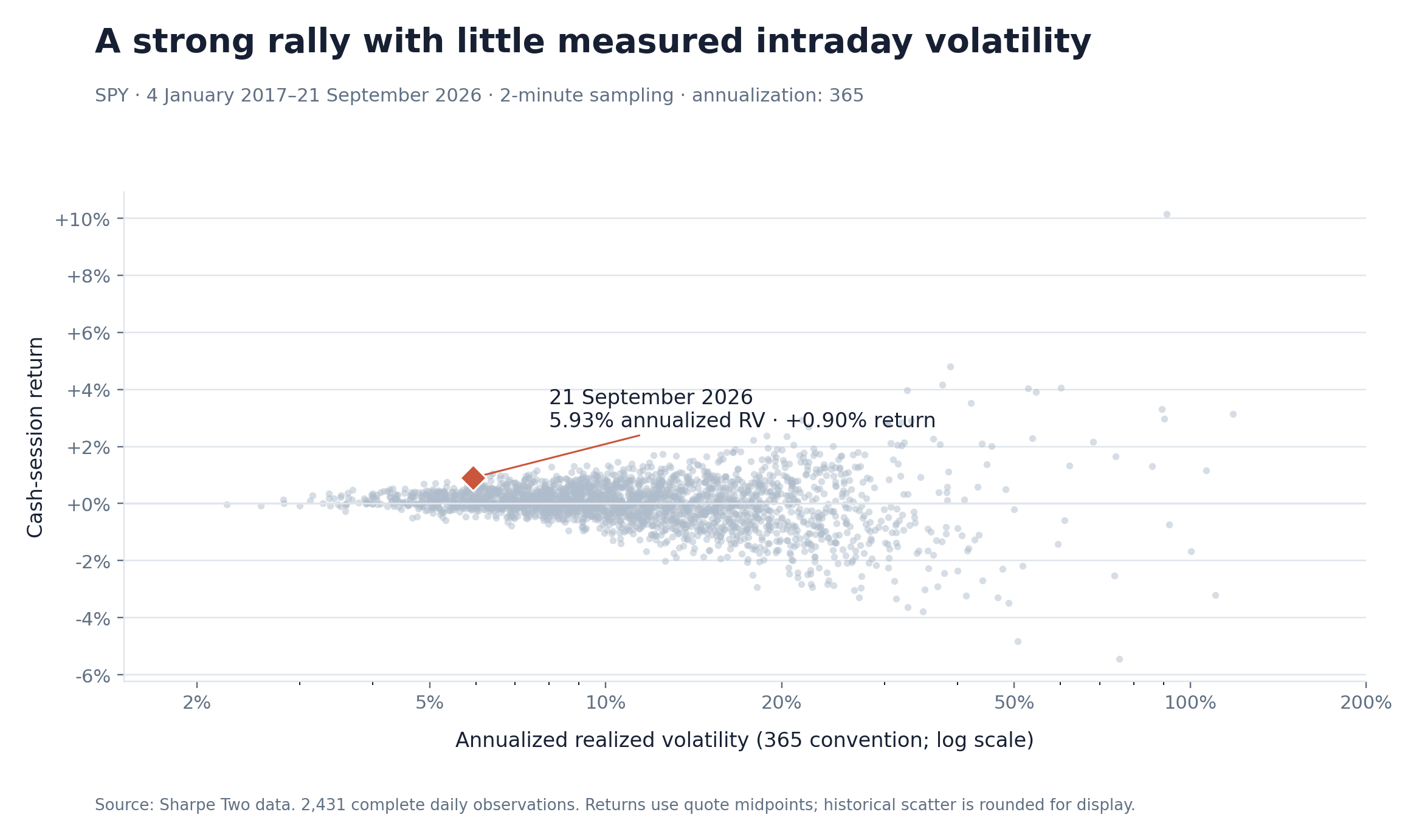
SPY gained 1.56% on 21 September. The more interesting number was what happened after the open: a 0.90% rise with just 5.93% annualized intraday realized volatility.

Across 2,431 complete sessions in our history, the return sits at the 91st percentile and the volatility at the 11th. No earlier session in that sample combined an intraday gain at least as large with realized volatility as low.

That is an unusual day. The harder question is whether it tells us anything useful about the next one.

How can a big rally have low volatility?

Return measures where the market ended relative to where it started. Realized volatility measures the size of the individual price changes along the way.

A succession of small upward moves can add up to a substantial gain. Squaring those small moves and adding them together can still produce a low realized-variance number. A market that repeatedly jumps up and down can do the opposite: plenty of measured volatility, little net progress.

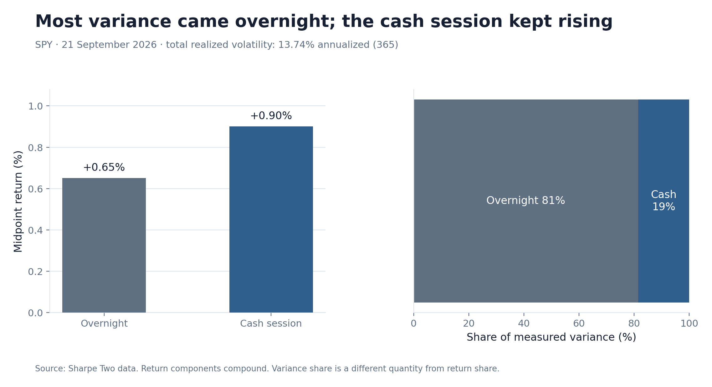
We use two-minute quote-midpoint returns here. On 21 September, about 0.65% of the gain came overnight and another 0.90% during the cash session. The overnight gap accounted for roughly 81% of measured close-to-close variance. Including it gives annualized realized volatility of 13.74%; looking only inside the session gives 5.93%.

To compare the cash-session return with its realized variation, both need to be on the same time scale. All annualized volatility in this article uses Sharpe Two’s 365 normalization:

Session realized variation = 5.925% ÷ √365 = 0.310%.

The 0.310% is the square root of the sum of squared two-minute log returns. It is the session’s measured variation before annualization—not a forecast of how far SPY should move, and not the square root of a volatility percentage.

Divide the session’s log return, 0.897%, by that 0.310% and the ratio is 2.89. It describes a large net gain relative to the variation accumulated along the sampled path. It is not a Sharpe ratio or a claim that this was a “2.89-sigma” event under a forecasting model.

On an absolute basis, that ratio is above 99.7% of observations in our sample. Five-minute sampling tells the same story: 6.08% annualized intraday volatility and a ratio of 2.82.

Was this positioning?

It could have been. A persistent buy program, short covering spread across the day, or a relatively thin supply of willing sellers could each help produce a steady advance. Gradual repricing of information could look similar.

The price-and-variance data cannot distinguish those explanations. Calling this a positioning squeeze would require evidence on flows, positioning or market depth that we have not used here.

What we can say is narrower: the session delivered unusually large net progress for its measured variation. There is no requirement for the price gain to reverse just because volatility was low. Neither number was “lying.” They describe different features of the same path.

What happened after comparable days?

We looked for earlier sessions with an intraday gain of at least 0.75% and annualized intraday volatility no higher than 7.22%. This is a comparison with similar historical days, rather than a forecast model fitted before the event.

There were 11 earlier dates.

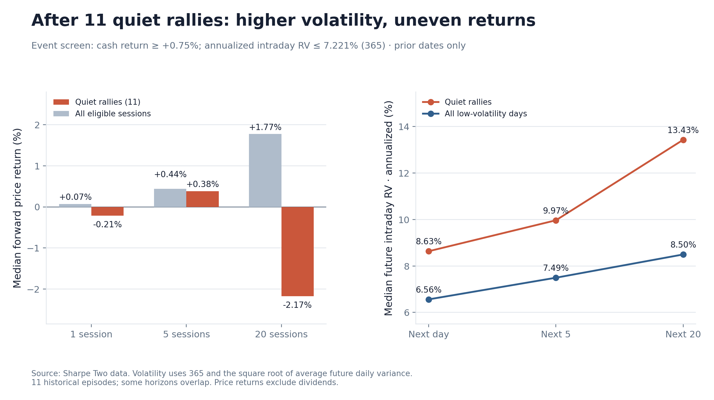
The clearest pattern was higher subsequent volatility. Median annualized intraday RV was 8.63% the next day, 9.97% over the next five sessions and 13.43% over the next 20. In all 11 cases, realized volatility over each of those horizons exceeded the event-day reading.

That supports a normalization interpretation. It does not automatically mean a return to turmoil: a rise from an exceptionally quiet session to roughly 9–10% annualized volatility is a meaningful increase from a low starting point. Low-volatility days in general also saw volatility rise, although their median next-20-session RV was lower, at 8.50%.

Returns were less consistent. The median was −0.21% after one session, +0.38% after five and −2.17% after 20, versus +1.77% over 20 sessions across the eligible historical baseline. These are midpoint price returns, excluding dividends.

The one-month figure deserves scrutiny, and so does its sample size. Five of the 11 outcomes were positive. December 2021 and July 2024 were followed by losses of roughly 9.0% and 7.6%; April 2026 was followed by a 6.3% gain. Similar-looking sessions led to very different paths.

Removing overlapping 20-session episodes leaves nine observations and the same −2.17% median. But modest changes to the screen change the result substantially: allowing RV up to 7.5% gives 18 observations and a −0.35% median; allowing 8% gives 25 and a +0.26% median.

The durable finding is volatility normalization. The one-month decline is interesting, but it changes too much with the definition of a comparable day to carry a bearish forecast on its own.

Could you spot it in SPY at noon and buy the afternoon?

That is the natural next question. We tested it with Sharpe Two’s intraday variance data.

At noon New York time, calculate the signed morning log return divided by the square root of morning realized variance. If it exceeds the 90th percentile of earlier eligible sessions, buy at 12:01 and exit at 16:00. Each threshold uses at least a year of prior observations. Exchange half-days are excluded.

This historical test uses two-minute sampling and runs through 18 September, before the session that prompted this article.

Across 223 signals, 54.7% of afternoons were positive and the median gain was 4.36 basis points. Yet the gross average was −1.87 basis points. That hit rate flattered the strategy: winning trades averaged about +0.30%; losing trades averaged −0.40%.

The uncertainty is wide: a month-block bootstrap puts the gross average’s 95% interval at roughly −8.70 to +4.52 basis points.

One-minute sampling at noon also produced a negative average. Waiting until 12:45 gave a small positive gross average. In SPY alone, the continuation evidence was inconclusive.

The more interesting result was in ETFs

We moved the observation time to 10:30 and expanded the test to stocks and ETFs. Compare each ticker’s cumulative return-to-variation score with its own earlier 10:30 readings. Enter at 10:31 if it is in the top decile, then look at what happens by the close. All results below use gross quote-midpoint price returns.

Across 32,849 signals in 164 ETFs, the average remainder-of-session return was +6.83 basis points. The median was +6.89 basis points, and 54.5% of outcomes were positive.

The same ETFs on non-signal days averaged −1.20 basis points, weighted to match their representation in the signal sample. That puts the difference at +8.03 basis points, with a month-block 95% confidence interval of +3.32 to +12.48. Comparing against non-qualifying ETFs on the same dates gives a similar +7.43-basis-point difference. The first comparison holds ETF identity constant; the second holds the date constant. Both point in the same direction.

The equity curve is worth seeing. Split the portfolio equally among qualifying ETFs each morning, close everything at 16:00, and reset the allocation the next day. From January 2018 through 18 September 2026, 100 becomes 230.9: a 10.1% CAGR, with a 30.9% maximum day-end drawdown. Buying all eligible ETFs over the same daily window, without the signal, leaves 86.4.

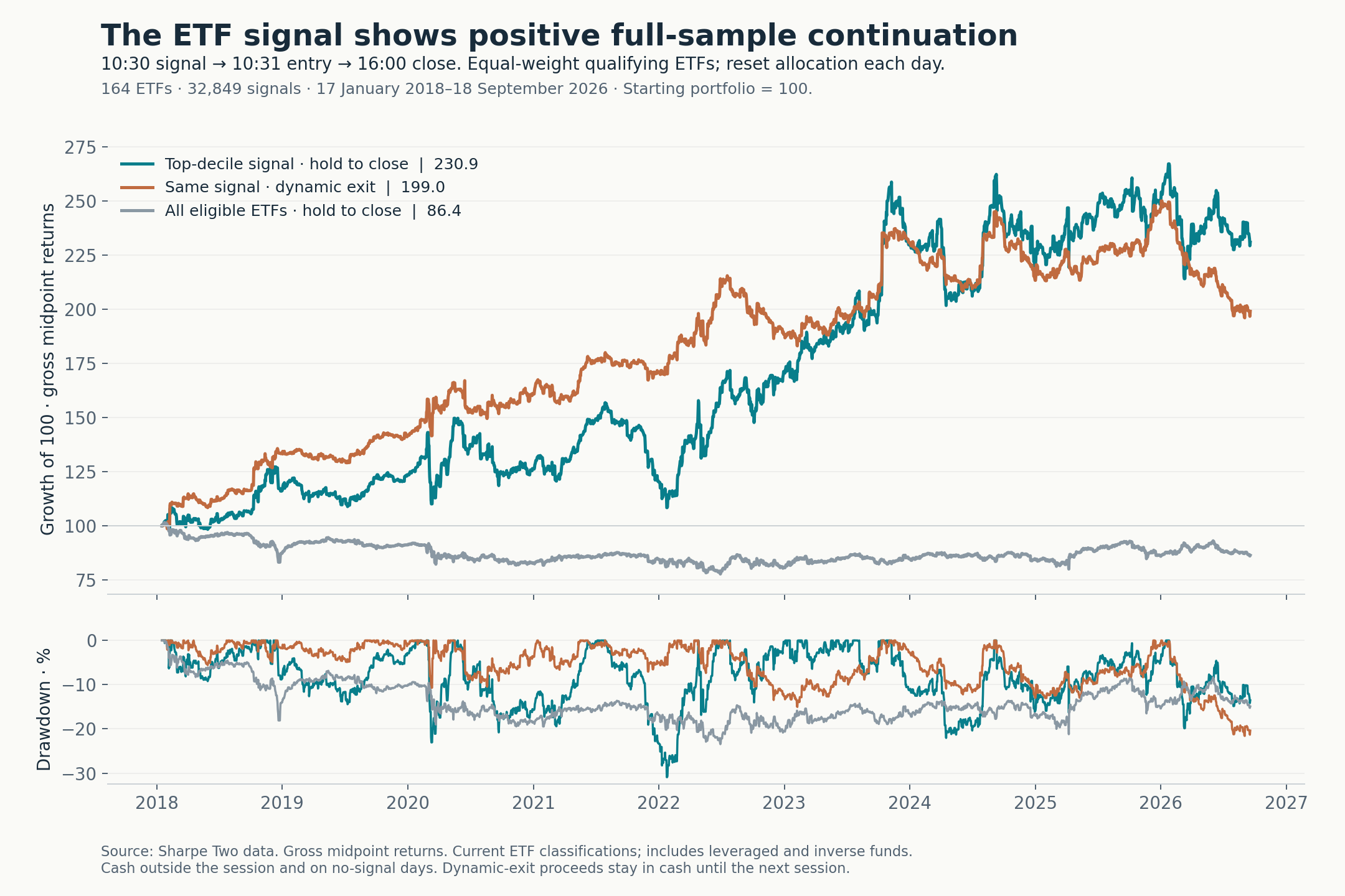
We also tried leaving when the signal faded: check every half-hour, exit one minute after the first failed check, and keep the proceeds in cash. That curve finishes at 199.0. It captures less return but has lower volatility, a smaller 21.6% drawdown, and a higher full-sample Sharpe: 0.68 versus 0.58. A smaller average gain does not, by itself, make the exit useless.

Nor is one ETF doing all the work. Removing the five largest contributing funds leaves a +5.83-basis-point mean. Excluding 40 funds whose current names explicitly indicate leverage or inverse exposure leaves +5.03 basis points across 124 ETFs. The corresponding stock test was less striking: 784 stock tickers averaged +1.78 basis points when held to close, versus +1.07 with the dynamic exit.

This is where the distinction between a signal and a trade matters. The signal describes a morning price path associated with stronger afternoon returns. Position sizing, overlapping fund exposures and exit timing determine how that information becomes a portfolio. The two curves use exactly the same entries; changing the exit already changes the risk profile substantially.

The result is not equally strong in every period: later-period confidence intervals include zero, and the hold-to-close curve lost 7.9% in 2026 through 18 September. This is a retrospective sample using current fund classifications and complete-session data, including leveraged and inverse ETFs. The next research question is specific: how much does the variation-adjusted score add beyond plain morning momentum, and in which market states?

The SPY session and the ETF result answer different questions. An exceptionally smooth SPY rally has historically been followed more consistently by higher volatility than by a price reversal. Across ETFs, a strong, smooth first hour was associated with a stronger afternoon. A large return and low realized volatility are not contradictory. Together, they describe a market state worth measuring.

Every figure and chart in this article was built with Sharpe Two data. Explore the S2 API to bring that data into your own research. For access and integration enquiries, get in touch with Sharpe Two.