Selling the SPY Volatility Spike: A Case Study

On Friday, October 16, the VIX opened at 16.02 and traded as high as 22.31. That was a 6.29-point move from the open. By the close, it was back at 19.99. Calculated from five-minute VIX returns, the session’s realized volatility was about 356% annualized. It was the highest reading across the 199 sessions in our 2026 data through that day—roughly four times the year’s median—and the sixth-highest across the 487 sessions in our data since the 2024 US election.

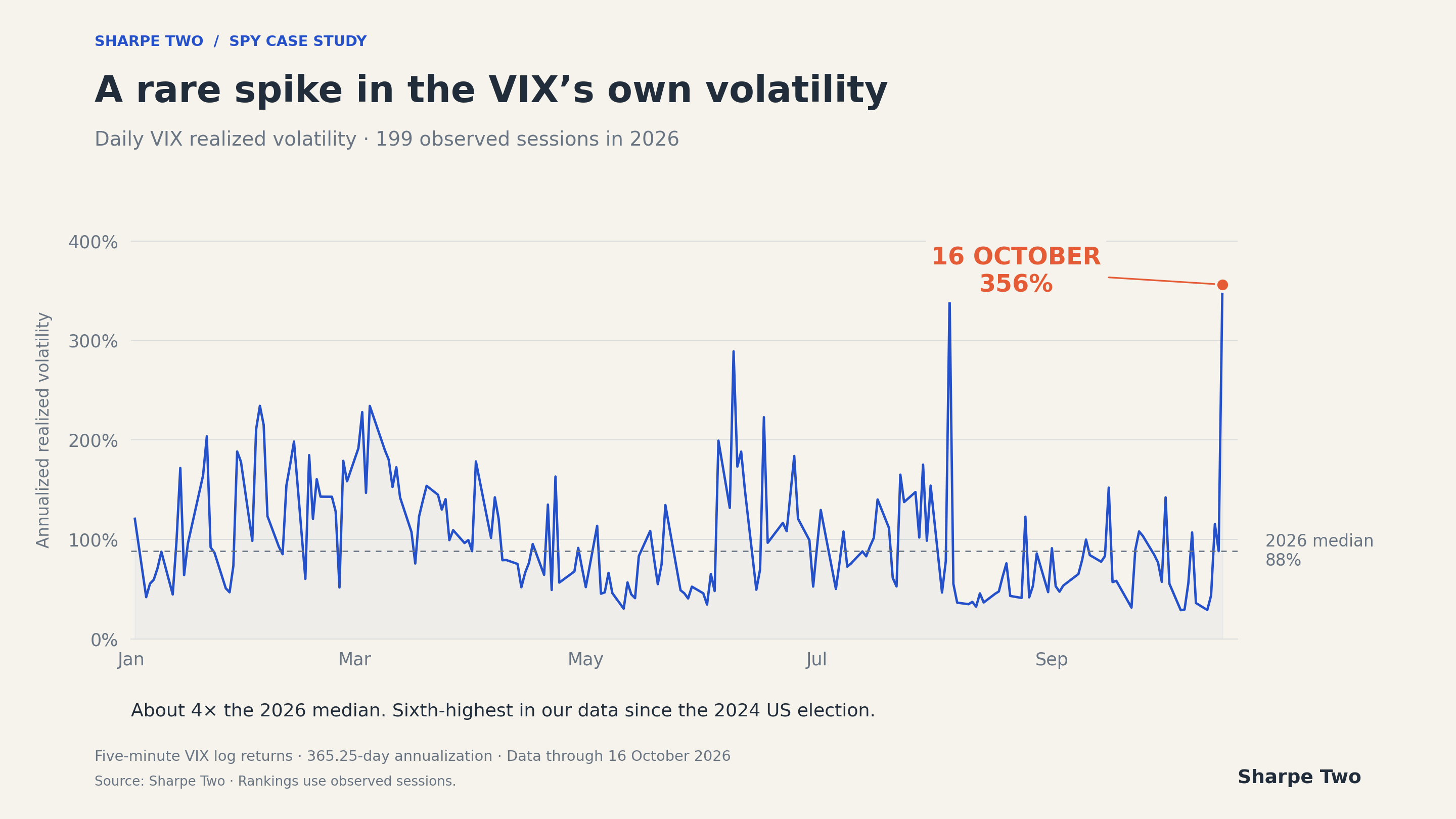
October 16 was the highest VIX realized-volatility reading among the 199 sessions in our 2026 data.

There was plenty of chatter to explain it. Speculation about a possible Israeli strike on Iran circulated alongside rumors that a fund was being liquidated. Each narrative offered a story about the move. None answered the question we actually needed to resolve: was it time to get active, and if so, how?

This is where agentic trading becomes useful. Social media can supply context, but it can also bury a decision under a pile of competing explanations. An agent with the right data can bring the discussion back to what the market is pricing and whether the opportunity is worth taking.

Our conclusion was that volatility was worth selling. The next question was which trade to use.

Why we wanted to sell the SPY volatility spike

Agentic trading means using an AI agent that can choose and call tools to carry out parts of a trading workflow. In this case, the useful work is gathering the data, comparing possible trades and helping us decide how to express a view.

The agent needs context: what is happening now, what the market expects, and what our forecasts and probabilities say about what may happen next.

Here is what the retained Sharpe Two SPY snapshots show:

MeasureOctober 15October 1630-day model-free implied volatility, at the bid16.0%19.6%Recent 30-day realized volatility10.6%10.5%Implied-minus-recent-realized spread5.4 points9.1 pointsProbability that implied exceeds subsequent 30-day realized volatility58.0%66.7%

The spread is expressed in annualized volatility points. Friday's snapshot showed the market charging substantially more for volatility while recent realized volatility remained near 10.5%. Our forward-looking probability also strengthened, reaching roughly two chances in three.

That was the basis for our view. We had a price gap and a forecast supporting the same direction. The Forward Note published that weekend discussed precisely this opportunity.

Regime matters here. An implied-volatility reading near 20 against recent realized volatility near 10 describes a different market from IV at 30 and RV at 20. The absolute gap may be similar, but the underlying is already moving much more in the second situation. The amount of exposure we want, the hedge we choose and our willingness to adjust should reflect that difference.

The term structure adds another piece of context. In the retained October 16 snapshots, 9-day bid implied volatility was 18.7% at 13:15, against 20.6% at 30 days and 21.0% at 61 days. At 15:45, those readings were 17.9%, 19.6% and 20.3%. The front had eased relative to the earlier snapshot, and these three tenors remained upward sloping.

Those are useful facts for an agent to work with. It can examine how the repricing is distributed across expiries and compare the cost of selling one part of the curve while buying another.

One view, three ways to express it

Once we have a view on volatility, the trade still needs to fit the portfolio. A strangle, a calendar and an iron condor can all involve selling options, but they give us very different exposures.

We see the human as the portfolio manager and the agent as the quant or trading assistant. The agent can assemble the comparison, but the final decision belongs to the human, who defines the objectives and makes the choice.

For the comparison below, we reconstructed the available SPY quotes from the October 16 snapshot labelled 15:45, with SPY at $762.09. We use November 20 options, 35 calendar days away, and December 18 options for the calendars. These are historical quoted examples, not a record of our execution prices. Entry credits use bids for options sold and asks for options bought.

1. The 20-delta strangle

The closest November 20 contracts to 20 delta were the 727 put and 790 call. Their deltas were approximately −0.202 and +0.195. Selling one of each at the displayed bids collected $8.53 per share, or $853 per one-lot strangle.

The put strike was 4.6% below SPY and the call strike 3.7% above it—a familiar expression of equity volatility skew, where demand for downside protection helps make puts more expensive in volatility terms. That is part of the appeal of this structure: the underlying has room to move between the two short strikes.

We tend to prefer 20-delta strangles when selling expensive volatility, particularly when we expect the market to move around but believe the insurance is overpriced.

An ATM straddle concentrates more vega and gamma near the current price. It can produce a larger gain when volatility falls and the underlying stays near the strike. As the underlying moves materially away, that vega exposure falls and the position becomes more directional. The strangle spreads the exposure across two strikes, which is the profile we prefer when we expect movement along the way.

Ultimately, we are betting that the market is overpaying, while allowing for the possibility that the underlying will move. After all, a VIX at 22 still tells us something about the market’s expectations of what may be coming next.

An agent can help make the choice explicit: do we want concentrated volatility exposure near the current price, or a broader profile that leaves more room for the underlying to move between the short strikes?

This is a useful assignment for the agent: show how the position's exposure changes as SPY moves, compare adjustment choices, and keep track of the limits we have set.

2. The ATM calendar

The alternative you might prefer is to sell a November option and buy a December option at the same at-the-money strike.

The nearest common strike was 762. A November 20/December 18 call calendar cost $6.04 per share, using the short call's bid and the long call's ask. The corresponding put calendar cost $4.47 per share.

The December option is there to cushion the position. If volatility rises across both expiries, its positive vega offsets part of the loss on the short November option. The calendar therefore carries much less exposure to a shared volatility shock than an outright short option; a conventional ATM long calendar will usually begin with positive net vega.

That is the trade-off we care about: we buy a hedge that can soften the swings in P&L, and give up some of the gain when the outright short-volatility trade works. We keep exposure to the difference between November and December, rather than remaining fully short the premium.

If SPY stays near the strike, faster decay in the front option will help the structure. Its path still depends on where SPY moves and how the two expiries reprice. The agent should show us that path alongside the strangle, so we can judge whether the extra hedge is worth paying for.

We tend to favor calendars when both implied and realized volatility are elevated and we want longer-dated options in the position. In the October 16 setup, our preference was to retain more of the short-volatility exposure through a strangle. The premium we were being paid was attractive relative to the recent movement in the underlying.

An agent equipped with the full surface can make this comparison concrete: what are we paying for the December leg, what happens if front and back volatility move differently, and how does the position behave if SPY moves away from the strike?

3. The iron condor

An iron condor is a familiar choice for traders who want to cap the position's expiry loss. We take the short strangle and buy a further-out put and call in the same expiry.

To make the cost visible, use the nearest available contracts to 10 delta as illustrative wings: the 690 put and 800 call. Buying those wings at the ask cost $4.27 per share. Against the strangle's $8.53 credit, that left $4.26, or $426 per one-lot condor.

The wings consumed about half the premium collected. In exchange, this particular combination capped its larger expiry loss at $3,274, before fees. Its widths were unequal: 37 points on the put side and 10 on the call side. Different wing choices would change both the credit and the loss limit.

The volatility prices tell a more interesting story than the dollar premiums alone. The short 727 put carried 20.3% IV, while the long 690 put carried 26.2%. We were buying the downside wing at substantially higher implied volatility. On the call side, the relationship ran the other way: 11.5% on the long wing against 12.0% on the short call.

That is why the agent needs strike-level data. It should show us which protection is expensive, how much premium it consumes and what exposure we receive for the cost.

We have written more about this in Why Iron Condors Eat Your Own Edge. Condors have a place, especially when the account or the trader requires a defined expiry loss. For small accounts, we tend to prefer the ATM calendar: buying the back month gives us the longer-dated hedge we want, while the condor’s wings can absorb a large share of the premium we are trying to collect.

In the end, our preference in this setup was the strangle; if we wanted a longer-dated option hedge, the ATM calendar deserved a comparison on its own terms.

What happened over the next twelve days?

By the October 28 snapshot, SPY was at $771.285, 1.2% above the entry snapshot. Its 30-day model-free implied volatility had fallen from 19.75% to 16.56%, a decline of about 3.2 volatility points, measured at the midpoint on both dates. We can reprice the same contracts to see how these choices developed.

The following comparison uses midpoint prices at both dates, one contract per leg, and no intervening adjustments. These are interim mark changes before costs; the positions have different capital requirements and exposures.

The same one-lot positions, marked at 15:45 each day. The calendars followed a steadier daily path while the strangle captured the larger dollar gain.

StructureOctober 16 entry markOctober 28 markChange per one-lotNovember 727/790 short strangle$859 credit$546 to close**+$313November/December 762 call calendar$592.50 debit$660.50 value+$68November/December 762 put calendar$433.50 debit$508 value+$74.50Illustrative 690/727/790/800 iron condor$435.50 credit$316 to close+$119.50**

The strangle produced the largest dollar gain per one-lot over this interval. Its put fell from a midpoint of $5.545 to $2.105, while the call rose from $3.045 to $3.355. The gain on the put more than offset the loss on the call.

The calendars also increased in value. They gave us a different exposure and earned less in dollars in this reconstruction. The condor retained a smaller gain after the change in the value of its wings.

What drove the strangle’s profit?

We applied Sharpe Two’s attribution calculation to daily 15:45 snapshots of the two options, matching the entry and exit marks in the comparison above.

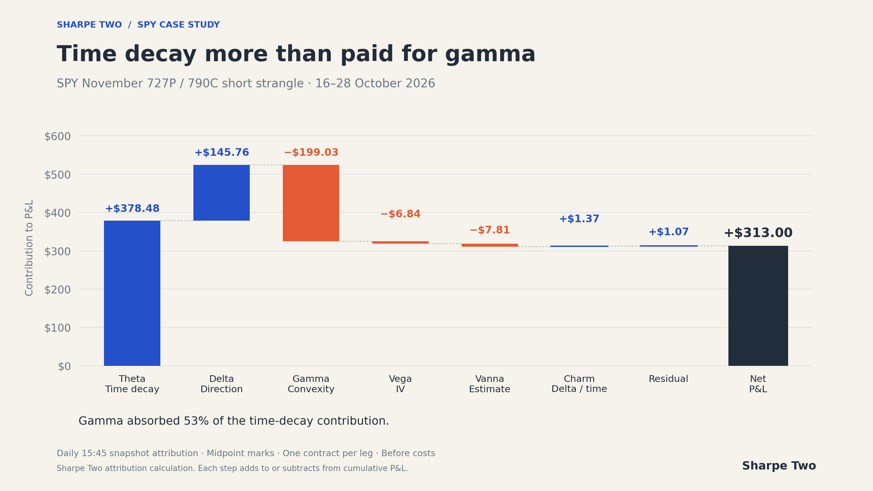
Time decay more than covered the gamma drag. Each Greek remains visible in the daily-snapshot attribution.

Theta did the heavy lifting. Time decay contributed $378.48 as the short options moved closer to expiry. That income paid for the exposures we were carrying.

Gamma was the largest drag. A short strangle’s delta changes against us as the underlying moves: a rally leaves the position more negatively exposed, while a fall leaves it more positively exposed. Those changes cost $199.03 in this daily calculation. Delta contributed $145.76, so the combined effect of price movement was a loss of about $53. This is why the path matters, even when the underlying finishes between our strikes.

Vanna also reduced the gain. Our volatility exposure changed as the options moved around the surface. A one-point change in IV therefore did not hit the same amount of vega throughout the trade. The model estimates vanna from observed changes in SPY, each option’s vega and its IV along the path. It allocated a $12.93 cost to the put, partly offset by a $5.12 gain on the call, for a net cost of $7.81.

Theta more than covered the gamma drag, and the trade remained profitable after the other contributions. That is the balance we wanted from selling the spike: collect enough premium for the movement we had to absorb. An agent should make that balance visible: how much did we earn from carrying the position, what did gamma and vanna take back, and how would a different structure change that trade-off?

Sharpe Two’s MCP gives the agent access to P&L attribution. Give it the contracts and holding period, ask for the Greek-by-Greek breakdown, then use the result to compare the exposure you held with the alternatives you considered.

That gives the discussion a concrete answer. Our preference for the strangle meant keeping more exposure to the opportunity we saw. Buying protection changed both what we could earn and how the position could lose. An agent's job is to make that trade-off visible before we choose.

Give your agent the context to challenge you

With the right data, an agent can take an active part in deciding how to express a view. It can compare the strangle, calendar and condor against the same market snapshot and the same portfolio objectives. It can also challenge a proposal that does not fit the evidence.

Without that context, a fluent answer can still be a poor trading answer. The agent can hallucinate an explanation, repeat a familiar strategy or agree too readily with the trade we already wanted to make.

Our contribution at Sharpe Two is the research behind that conversation: forecasts, probabilities and options analytics that help humans and agents assess an opportunity. Your agent becomes more useful when it has something substantial to reason from.

Try Sharpe Two's forecasts and probability signals and put them to work on your next trading idea. Or start with VRP Central to compare implied and recent realized volatility for an underlying you follow.