Why you need an opinion on future realized volatility

If you sell options and have ever put implied volatility next to recent realized volatility and thought "these look expensive," you have already made a forecast. You just haven't said it out loud. Implied volatility tells you how the option is priced today. Whether that price is rich depends on how much the underlying will actually move over the life of the option, and nobody can observe that yet. Using last month's realized volatility as the yardstick quietly assumes the next month will look like the last one.

That assumption is often reasonable. It is still an opinion about future realized volatility. Once you see it that way, the obvious next question is whether you can form a better one.

What an option premium pays for

A protective put is the clearest way to see what an option premium pays for. You own a stock, you like the upside, and you would rather not carry the full downside. So you buy a put. Like a home or car insurance policy, you pay a premium so that someone else absorbs part of the loss if things go badly.

The seller on the other side is acting a bit like an insurer. They take on a risk the buyer wants to get rid of, commit capital and occasionally pay a large claim. They expect compensation for that service. The practical question is whether the premium on offer adequately compensates them for the risk.

Take a stock you buy at $100. You like its upside but want protection against a large fall. A put with an $80 strike puts a floor under the position at expiry: the stock and put together will be worth at least $80 per share. Your maximum loss is $20 per share plus the premium paid. The strike decides where the protection starts. The premium is what it costs. So how much should that premium be?

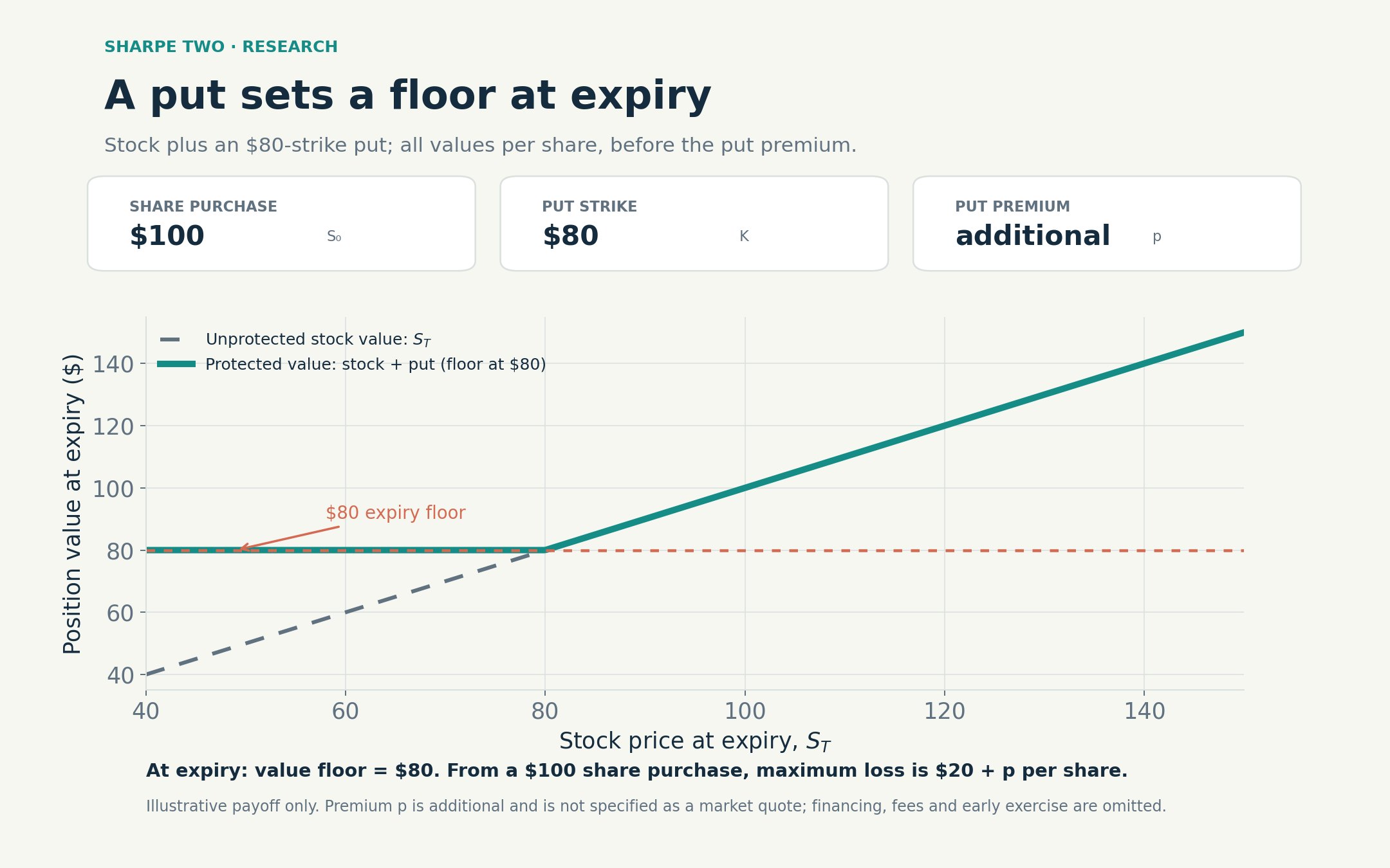
A protective put sets a floor at expiry. With the stock bought at $100 and an $80 strike, the maximum loss is $20 per share plus the premium paid. Values shown are per share, before the premium.

What implied volatility actually measures

Option pricing models, Black-Scholes being the classic one, take inputs including the underlying price, strike, time to expiry, interest rates, dividends and a key assumption: volatility. The more volatile a stock, the wider the range of prices it could reach at expiry. That makes the downside protection more valuable. All else equal, the insurance should cost more.

Given the other inputs and assumptions, we can work backwards from an observed option price. Implied volatility is the volatility number that makes the model reproduce that price (OIC explains the pricing inputs).

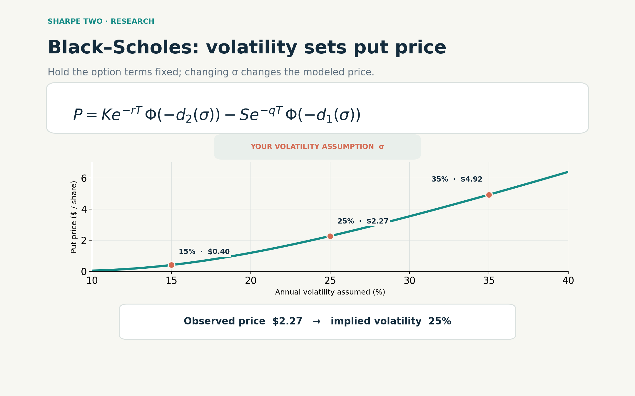
Hold the other inputs fixed: more assumed volatility raises the put price. Reading the curve backwards gives implied volatility. Example: stock $100, strike $80, one year to expiry, zero rates and dividends; prices are per share.

That makes implied volatility a price expressed in volatility units. Expectations about future movement and compensation for taking risk both influence that price. Reading IV as an unbiased forecast of future realized volatility misses this distinction. Nor does a high IV automatically mean an option is expensive: it may be pricing a substantial risk.

For a seller, the question is how the volatility priced into the option compares with the movement they expect over its life. That requires an estimate of something that has not happened yet.

The seller has to get that estimate right enough to quote a sensible premium. In this simple example, an unhedged seller who holds to expiry and collects less than the expected payout has a negative expected profit before costs. Charge much more than another seller offering the same protection and the buyer may go elsewhere. The illustration below makes that trade-off concrete under a simple set of assumptions.

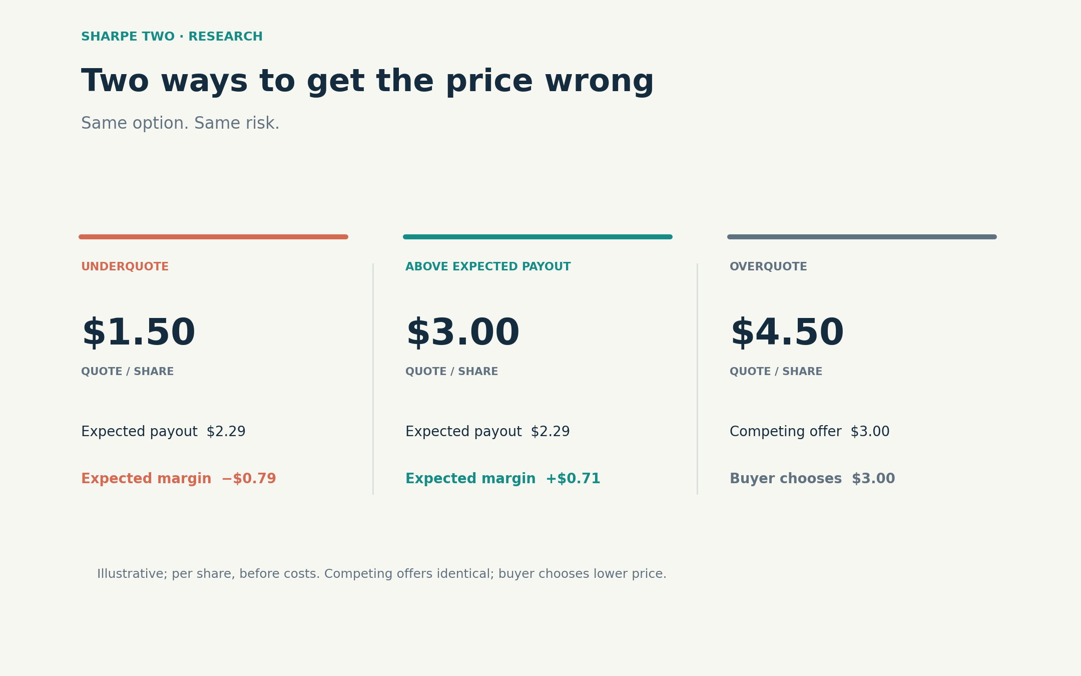
Illustrative 30-day, at-the-money put on a $100 underlying. Under a lognormal model with 20% annual volatility, zero expected stock return, and zero interest rates and dividends, the expected expiry payout is $2.29 per share. Margins exclude costs; competing offers are identical and the buyer chooses the lower price.

Using recent realized volatility as a guide

The usual shortcut compares implied volatility with recent realized volatility. When implied sits well above realized, options can look expensive. There is a reason for using this shortcut: volatility clusters. Calm periods tend to follow calm periods, and turbulent ones follow turbulent ones. A little like the weather in continental Europe: if it rained today, rain tomorrow is a decent bet.

The forward-looking variance risk premium compares model-free option-implied variance with expected future realized variance over the same horizon (the Federal Reserve describes this distinction). Variance is volatility squared, and the comparison needs consistent units and time conventions. Using recent realized variance as the expectation is the persistence assumption from the opening. The historical spread is a useful starting point; it does not tell us what will happen next.

You can explore implied and realized volatility in our free VRP Central tool.

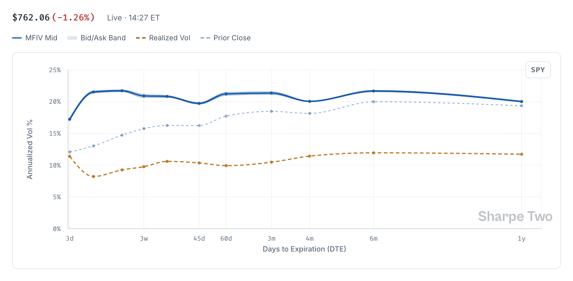
SPY in VRP Central on 16 October 2026 at 14:27 ET. Solid blue: current model-free IV. Dotted blue: prior close. Orange: realized volatility. The horizontal axis is days to expiry.

In this snapshot from Friday, 16 October 2026, SPY was down 1.26% and implied volatility was above its prior close across the displayed expiries. The repricing was strongest at shorter expiries. That jump in IV can look inviting to an option seller, especially with historical realized volatility still much lower. But the market may be anticipating turbulence that recent returns cannot show yet. We need a forecast to assess whether the richer premium adequately compensates us for the movement ahead.

From today's weather to a forecast

Persistence is a useful baseline. It is still an assumption. Rain today makes rain tomorrow more likely, and you would still check the forecast before planning a weekend outside. Volatility works the same way. Scheduled earnings, macro releases, a shock that is fading, the shape of the term structure: there is information beyond last month's returns about how much the market is likely to move over the life of an option.

There is a large literature on this problem. GARCH models use recent shocks and variance to estimate future variance. Corsi's HAR model combines realized volatility over daily, weekly and monthly windows. Both provide established benchmarks for more flexible methods. Additional complexity needs to earn its place on genuinely out-of-sample data, at the horizons that matter for the trade.

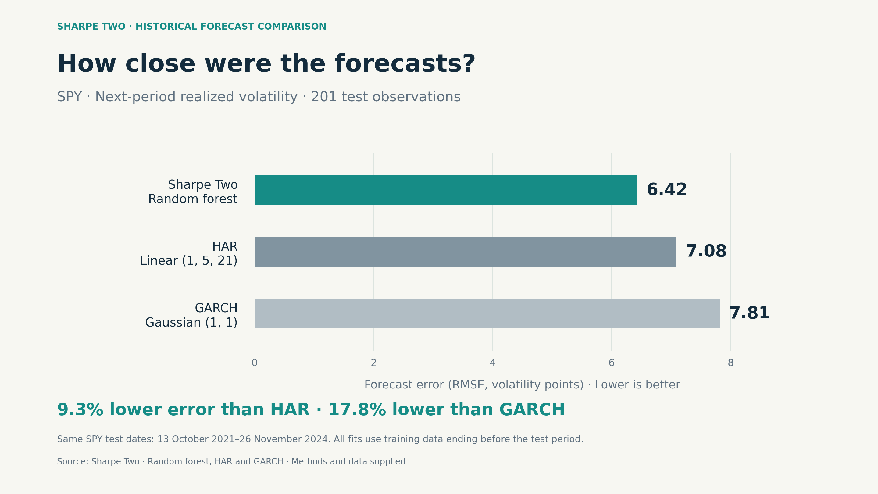
Across the same 201 sampled SPY forecast dates from October 2021 to November 2024, Sharpe Two’s random forest recorded an RMSE of 6.42 volatility points for the following trading period, versus 7.08 for linear HAR and 7.81 for GARCH—9.3% and 17.8% lower, respectively. Lower RMSE means a smaller forecast error.

The aim is to improve our estimate of risk over the life of the option, so we can judge the premium against the period we will actually be exposed to.

What we forecast, and what a probability means

At Sharpe Two we combine more than 50 features to forecast realized volatility over horizons from the next day out to 100 days. The value of those inputs depends on whether they improve the forecast out of sample. Think of us as a weather forecaster for the market. These forecasts concern how much the market may move, rather than whether it goes up or down.

A forecast is more useful with its uncertainty attached, which is why we also express views as probabilities. For example, we can ask how likely our model considers realized volatility to come in below the option-implied level over a specified future period. That can form the basis of a trade: a forecast of lower realized volatility than today’s implied level, measured over the same horizon and with consistent annualization, points to a potential volatility edge. We still need to weigh the size and uncertainty of that gap, tail risks and trading costs before choosing a structure to express the view.

That probability is different from the probability that your trade makes money. A short strangle and a cash-secured put can use the same volatility forecast and produce different outcomes. Payoff shape, direction, the price path, hedging and costs all affect P&L. Our forecasts and probabilities help assess the premium; our signals and strategies help connect that assessment to a trading decision.

Forecasts in an agentic workflow

More traders now hand parts of their research to AI agents. An agent can read an option chain, summarize the news and write a convincing paragraph on why premiums look rich. However, AI agents can struggle to identify and establish an edge, particularly when they are asked to rebuild datasets and analytics from scratch. The end user wants them to interpret reliable data and use those insights to assess a trade.

To assess a trade properly, an agent needs what a disciplined trader needs: a maintained quantitative forecast of realized volatility, probabilities with their event and horizon clearly defined, and the actual payoff of the position to evaluate them against. Without those inputs, it is reasoning about prices with no view on the risk underneath.

Whether you assess the trade yourself or use an agent to help, you need a view on the risk that will unfold after entry. Making that forecast explicit, understanding its uncertainty and checking its record gives you a firmer basis for judging the premium. That is the work we do at Sharpe Two.

Benchmark note: The comparison uses one historical random-forest specification trained across assets, with SPY-only HAR and GARCH baselines. All three use the same test dates and target; model parameters use training data ending before the test period. These retrospective results measure following-period forecasts, not live trading performance or every forecast horizon. The saved records do not establish that the test set was untouched during model selection.